TX RSB Improvement by IQ Calibration

Residual sideband suppression (RSB) is one of key TX specs. We want to minimize this because this degrades EVM (when LO is centered to CC leading to signal and its image falling on top of each other) or degrades ACLR (when LO is not centered to CC leading to different signal and image locations). Mismatches in amplitude or phase of I and Q channels in IQ TX generate RSB. Therefore, IQ correction is a usual calibration routine that is followed in industry practice where IQ errors are measured and corrected. We discuss below how it is done in context of TX.

Ideal IQ TX with No Mismatch

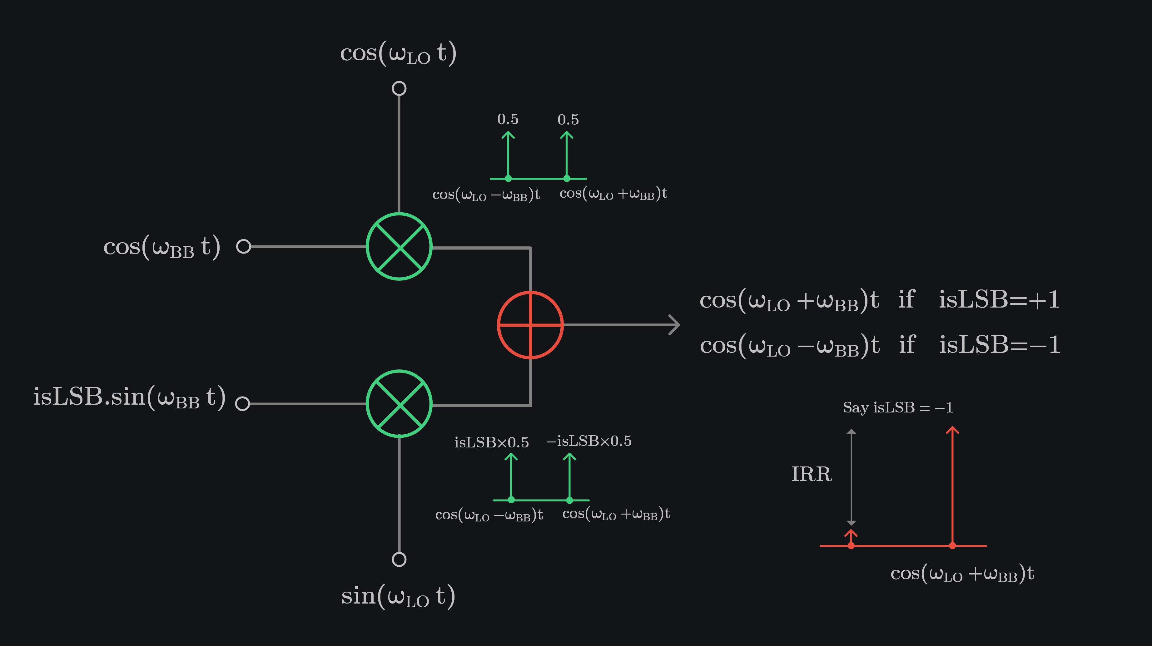
Consider an ideal IQ TX. I channel receives a cosine baseband signal from DAC and multiplies it with cosine LO. Q channel receives a sin baseband signal from DAC and multiplies with sin LO. Multiplication generates two sidebands: \(\omega_{LO}+\omega_{BB}\) aka upper sideband (USB) and \(\omega_{LO}-\omega_{BB}\) aka lower sideband (LSB). When I and Q are summed, one of the sideband cancels. Depending on the sign of “isLSB” (shown in image below), either lower sideband or upper sideband is transmitted, and the one that is cancelled is then called as residual sideband or image. The ratio of residual sideband to transmitted sideband is called as image rejection ratio (IRR). IRR is infinite in an ideal TX with no IQ mismatch.

IRR\;[dBc] = 10\;log \left[\frac{P_{RSB}}{P_{SIG}}\right]

where P_RSB is RSB power and P_SIG is signal power.

IQ TX with Gain and Phase Mismatch

Let \(\large \textcolor{#FEDB39}{\epsilon}\)\( \; \& \; \textcolor{#FEDB39}{\varphi} \) be the gain and phase mismatch (in radians) between I and Q channels. We can either scale I channel or Q channel to represent gain mismatch. Similarly, we can either add phase shift in I channel or Q channel (LO path or BB path) to represent phase error. The outcome is going to be the same i.e., a given gain and phase mismatch would give a certain RSB no matter where it comes from. Let’s scale the I-channel and add phase shift in Q LO path as shown in image below.

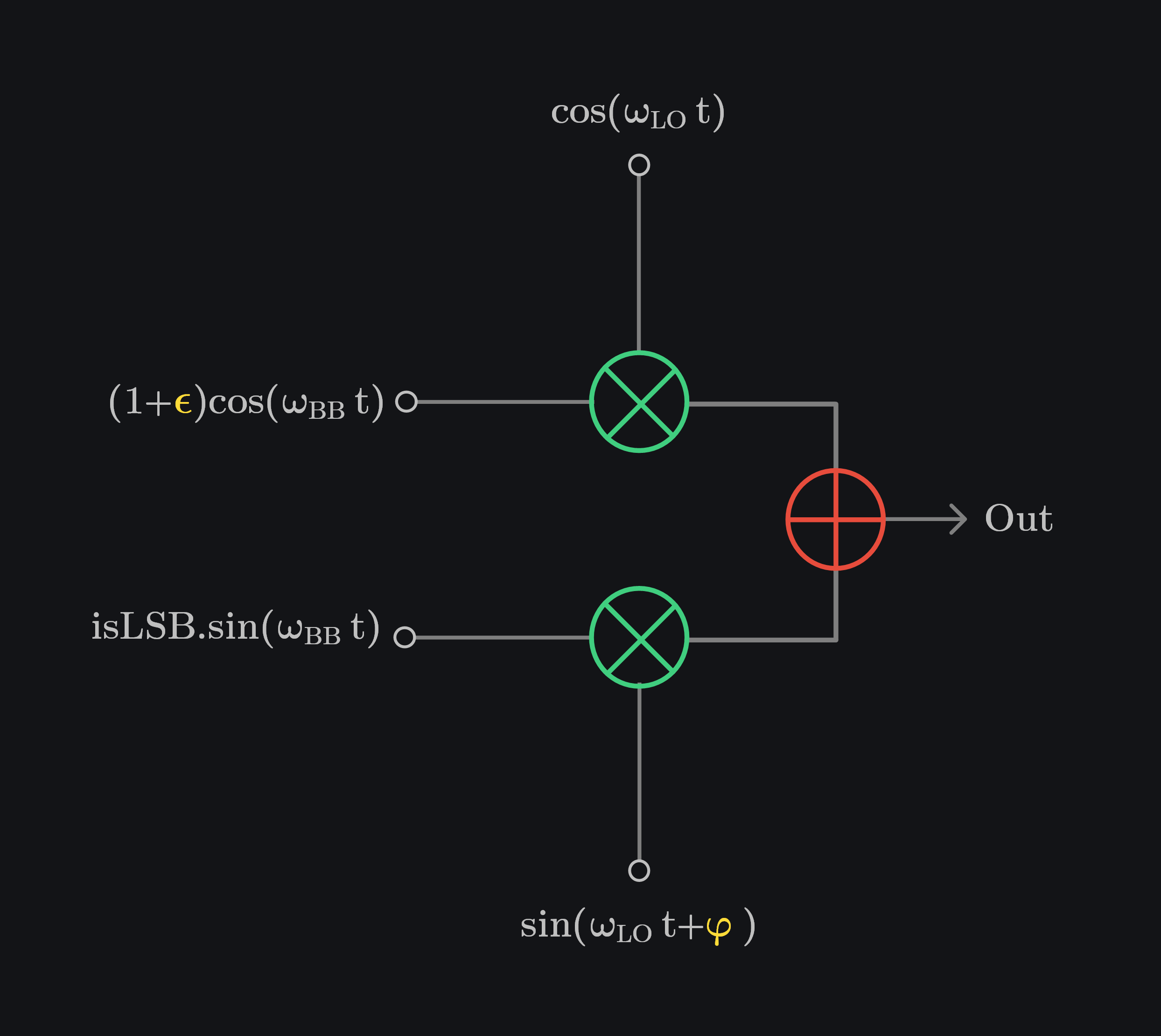
We can write output as follows:

Out = \overbrace{\frac{1+{\large \textcolor{#FEDB39}{\epsilon}}}{2} \biggr[ cos(\Sigma) + cos(\Delta)\biggr]}^{\text{I Channel}} +\overbrace{\frac{isLSB}{2} \biggr[ cos(\Delta+\textcolor{#FEDB39}{\varphi}) - cos(\Sigma+\textcolor{#FEDB39}{\varphi})\biggr]}^{\text{Q Channel}}

where \(\Sigma = (\omega_{LO}+\omega_{BB})t\) and \(\Delta = (\omega_{LO}-\omega_{BB})t\)

\begin{alignat*}{4} \Sigma \text{ Tone}&: \frac{1}{2}& \biggr[ (1+{\large \textcolor{#FEDB39}{\epsilon}}) cos(\Sigma) -isLSB.cos(\Sigma+\textcolor{#FEDB39}{\varphi)} \biggr]\\ \Delta \text{ Tone}&: \frac{1}{2}& \biggr[ (1+{\large \textcolor{#FEDB39}{\epsilon}}) cos(\Delta) +isLSB.cos(\Delta+\textcolor{#FEDB39}{\varphi)} \biggr] \end{alignat*}

Let’s take squares of these tones since we are interested in ratios of their powers.

$$ \text{Given: } |acos(\Sigma)+bcos(\Sigma+\varphi)|^2 = a^2+b^2+2ab\,cos(\varphi)\;\;\text{(see appendix)}$$ \begin{alignat*}{4} |\Sigma \text{ Tone}|^2 :& \frac{1}{4}& \biggr[ (1+{\large \textcolor{#FEDB39}{\epsilon}})^2-isLSB \cdot 2(1+{\large \textcolor{#FEDB39}{\epsilon}})cos(\textcolor{#FEDB39}{\varphi})+1 \biggr]\\ |\Delta \text{ Tone}|^2 :& \frac{1}{4}& \biggr[ (1+{\large \textcolor{#FEDB39}{\epsilon}})^2+isLSB \cdot 2(1+{\large \textcolor{#FEDB39}{\epsilon}})cos(\textcolor{#FEDB39}{\varphi})+1 \biggr] \end{alignat*}

If isLSB = -1, that is when we want to keep \(\Sigma\) tone and reject \(\Delta\) tone, IRR will be given as:

IRR = \frac{|\Delta \text{ Tone}|^2}{|\Sigma \text{ Tone}|^2} = \frac{(1+{\large \textcolor{#FEDB39}{\epsilon}})^2- 2(1+{\large \textcolor{#FEDB39}{\epsilon}})cos(\textcolor{#FEDB39}{\varphi})+1}{(1+{\large \textcolor{#FEDB39}{\epsilon}})^2+ 2(1+{\large \textcolor{#FEDB39}{\epsilon}})cos(\textcolor{#FEDB39}{\varphi})+1}

If isLSB = +1, that is when want to keep \(\Delta\) tone and reject \(\Sigma\) tone, IRR will be given as:

IRR = \frac{|\Sigma \text{ Tone}|^2}{|\Delta \text{ Tone}|^2} = \frac{(1+{\large{\textcolor{#FEDB39}{\epsilon}}})^2- 2(1+{\large{\textcolor{#FEDB39}{\epsilon}}})cos(\textcolor{#FEDB39}{\varphi})+1}{(1+{\large{\textcolor{#FEDB39}{\epsilon}}})^2+ 2(1+{\large{\textcolor{#FEDB39}{\epsilon}}})cos(\textcolor{#FEDB39}{\varphi})+1}

That means IRR is same no matter what sideband we transmit which makes sense since IRR should only be dependent upon gain and phase error.

Measurement of Gain and Phase Error

Simplification of IRR Equation

We want to make some measurements to evaulate \({\large \textcolor{#FEDB39}{\epsilon}}\)\( \; \& \; \textcolor{#FEDB39}{\varphi} \). These variables are tied together in IRR equation and not separable. We would need numerical techniques to solve this equation, therefore we want to simplify the equation to make IQ calibration easy and intuitive.

Assume \({\large \textcolor{#FEDB39}{\epsilon}} <<1\)\( \; \& \; \textcolor{#FEDB39}{\varphi} <<1 rad\). Let’s look at the denominator of IRR equation:

(1+{\large{\textcolor{#FEDB39}{\epsilon}}})^2+ 2(1+{\large{\textcolor{#FEDB39}{\epsilon}}})cos(\textcolor{#FEDB39}{\varphi})+1\\ $$ $$ =1+{\large{\textcolor{#FEDB39}{\epsilon}}}^2+2{\large{\textcolor{#FEDB39}{\epsilon}}}+2cos(\textcolor{#FEDB39}{\varphi})+2{\large{\textcolor{#FEDB39}{\epsilon}}}cos(\textcolor{#FEDB39}{\varphi})+1 $$ $$\text{Since } \textcolor{#FEDB39}{\varphi}<<1\;\; \implies cos(\textcolor{#FEDB39}{\varphi}) \approx 1-\frac{\textcolor{#FEDB39}{\varphi}^2}{2}$$ $$\therefore 1+{\large{\textcolor{#FEDB39}{\epsilon}}}^2+2{\large{\textcolor{#FEDB39}{\epsilon}}}+2\left[1-\frac{\textcolor{#FEDB39}{\varphi}^2}{2}\right]+2{\large{\textcolor{#FEDB39}{\epsilon}}}\left[1-\frac{\textcolor{#FEDB39}{\varphi}^2}{2}\right]+1$$ $$=1+{\large{\textcolor{#FEDB39}{\epsilon}}}^2+2{\large{\textcolor{#FEDB39}{\epsilon}}}+2-\textcolor{#FEDB39}{\varphi}^2+2{\large{\textcolor{#FEDB39}{\epsilon}}}-{\large{\textcolor{#FEDB39}{\epsilon}}}\textcolor{#FEDB39}{\varphi}^2+1$$ $$=4+4{\large{\textcolor{#FEDB39}{\epsilon}}}+{\large{\textcolor{#FEDB39}{\epsilon}}}^2-\textcolor{#FEDB39}{\varphi}^2(1+{\large{\textcolor{#FEDB39}{\epsilon}}})$$ $$\approx 4 \;\;\because {\large{\textcolor{#FEDB39}{\epsilon}}}<<1

Doing similar manipulations on numerator:

(1+{\large{\textcolor{#FEDB39}{\epsilon}}})^2- 2(1+{\large{\textcolor{#FEDB39}{\epsilon}}})cos(\textcolor{#FEDB39}{\varphi})+1\\ $$ $$ =1+{\large{\textcolor{#FEDB39}{\epsilon}}}^2+2{\large{\textcolor{#FEDB39}{\epsilon}}}-2cos(\textcolor{#FEDB39}{\varphi})-2{\large{\textcolor{#FEDB39}{\epsilon}}}cos(\textcolor{#FEDB39}{\varphi})+1 $$ $$\text{Since } \textcolor{#FEDB39}{\varphi}<<1\;\; \implies cos(\textcolor{#FEDB39}{\varphi}) \approx 1-\frac{\textcolor{#FEDB39}{\varphi}^2}{2}$$ $$\therefore 1+{\large{\textcolor{#FEDB39}{\epsilon}}}^2+2{\large{\textcolor{#FEDB39}{\epsilon}}}-2\left[1-\frac{\textcolor{#FEDB39}{\varphi}^2}{2}\right]-2{\large{\textcolor{#FEDB39}{\epsilon}}}\left[1-\frac{\textcolor{#FEDB39}{\varphi}^2}{2}\right]+1$$ $$=1+{\large{\textcolor{#FEDB39}{\epsilon}}}^2+2{\large{\textcolor{#FEDB39}{\epsilon}}}-2+\textcolor{#FEDB39}{\varphi}^2-2{\large{\textcolor{#FEDB39}{\epsilon}}}+{\large{\textcolor{#FEDB39}{\epsilon}}}\textcolor{#FEDB39}{\varphi}^2+1$$ $$={\large{\textcolor{#FEDB39}{\epsilon}}}^2+\textcolor{#FEDB39}{\varphi}^2(1+{\large{\textcolor{#FEDB39}{\epsilon}}})$$ $$\approx {\large{\textcolor{#FEDB39}{\epsilon}}}^2+\textcolor{#FEDB39}{\varphi}^2 \;\;\because {\large{\textcolor{#FEDB39}{\epsilon}}}<<1

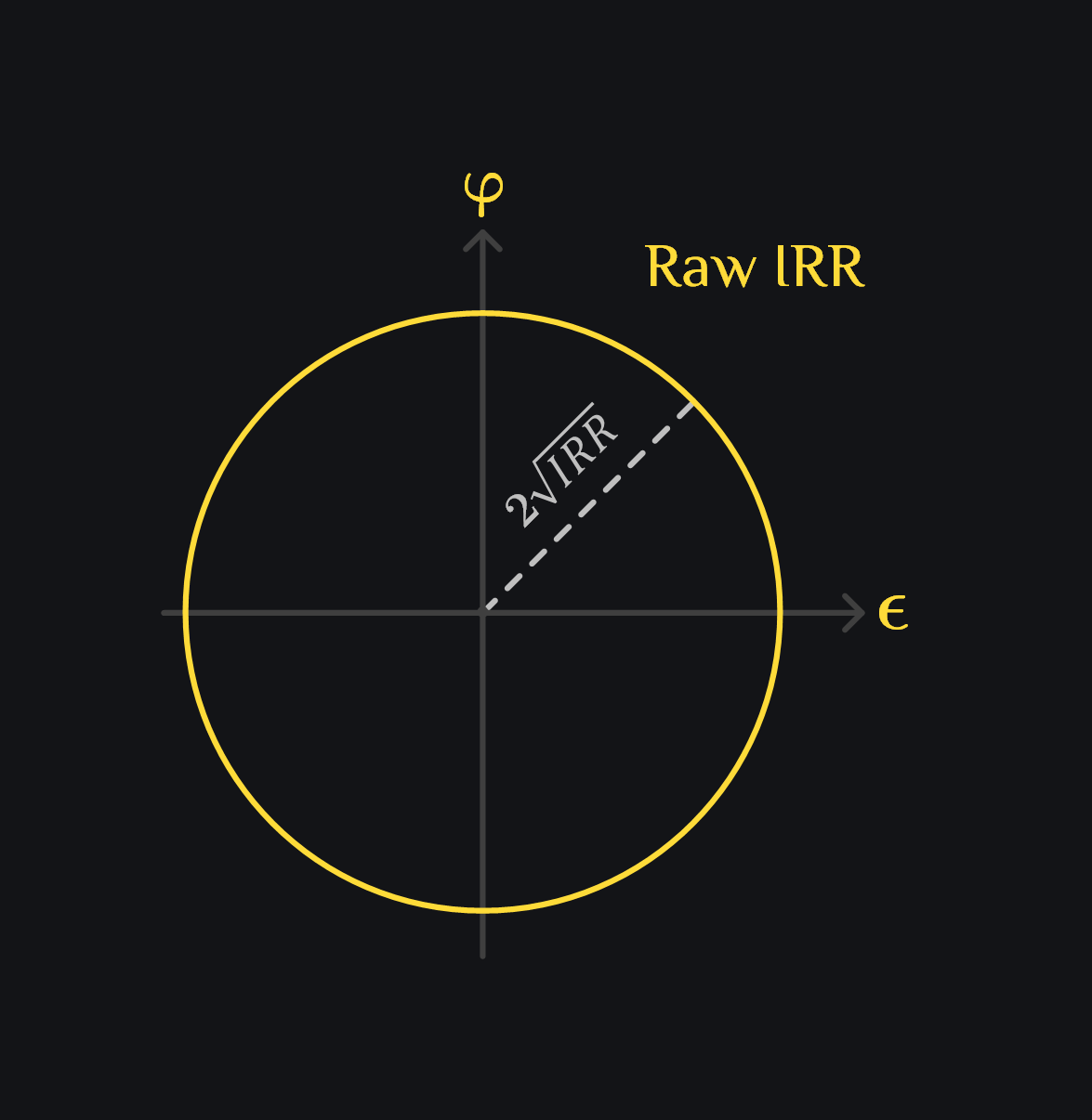
We can finally write IRR equation as follows:

IRR \approx \frac{{\large{\textcolor{#FEDB39}{\epsilon}}}^2+\textcolor{#FEDB39}{\varphi}^2}{4}$$ $$\implies 4 \cdot IRR \approx {\large{\textcolor{#FEDB39}{\epsilon}}}^2+\textcolor{#FEDB39}{\varphi}^2

which shows IRR is an equation of circle in plane of \({\large \textcolor{#FEDB39}{\epsilon}}\) and \(\textcolor{#FEDB39}{\varphi}\) with radius of \(2\sqrt{IRR}\). This means there can be different combinations of (\({\large \textcolor{#FEDB39}{\epsilon}}\),\(\textcolor{#FEDB39}{\varphi}\)) that will lead to same IRR.

IQ Calibration Algorithm

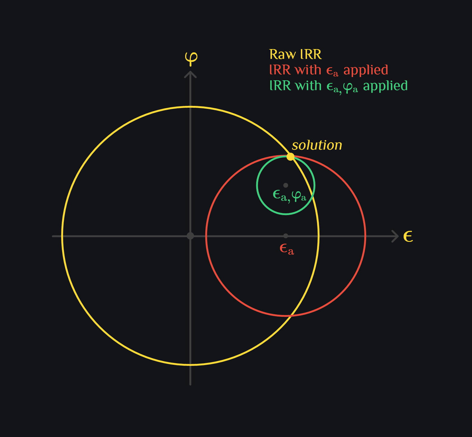
We can figure out \(\large \textcolor{#FEDB39}{\epsilon}\)\( \; \& \; \textcolor{#FEDB39}{\varphi} \) by applying some gain and phase errors ourselves and measuring resultant IRRs as proposed in [3].

Measure intrinsic \(IRR_1\). Draw the yellow circle with radius of \(2\sqrt{IRR_1}\) and center \((0,0)\). \({\large{\textcolor{#FEDB39}{\epsilon}}}^2+\textcolor{#FEDB39}{\varphi}^2 = 4 \cdot IRR1\) Apply a small gain error \({\large\epsilon_a}\) and measure \(IRR_2\). Draw an orange circle with radius of \(2\sqrt{IRR_2}\) and center \(({\large\epsilon_a},0)\) $$({\large{\textcolor{#FEDB39}{\epsilon}}}-{\large{\epsilon_a}})^2+\textcolor{#FEDB39}{\varphi}^2 = 4 \cdot IRR2$$ $${\large{\textcolor{#FEDB39}{\epsilon}}}^2-2{\large{\textcolor{#FEDB39}{\epsilon}}}{\large{\epsilon_a}}+{\large{\epsilon_a}}^2+\textcolor{#FEDB39}{\varphi}^2 = 4 \cdot IRR2$$ $${\large{\epsilon_a}}^2-2{\large{\textcolor{#FEDB39}{\epsilon}}}{\large{\epsilon_a}}+4 \cdot IRR1 = 4 \cdot IRR2$$ $${\large{\textcolor{#FEDB39}{\epsilon}}} = \frac{4(IRR1-IRR2)+{\large{\epsilon_a}}^2}{2{\large{\epsilon_a}}}$$ Apply gain error \({\large\epsilon_a}\) and small phase error \(\varphi_a\) and measure \(IRR_3\). Draw a green circle with radius of \(2\sqrt{IRR_3}\) and center \(({\large\epsilon_a},\varphi_a)\). $$({\large{\textcolor{#FEDB39}{\epsilon}}}-{\large{\epsilon_a}})^2+(\textcolor{#FEDB39}{\varphi}-\varphi_a)^2 = 4 \cdot IRR3$$ $${\large{\textcolor{#FEDB39}{\epsilon}}}^2-2{\large{\textcolor{#FEDB39}{\epsilon}}}{\large{\epsilon_a}}+{\large{\epsilon_a}}^2+\textcolor{#FEDB39}{\varphi}^2-2\textcolor{#FEDB39}{\varphi}\varphi_a+\varphi_a^2 = 4 \cdot IRR3$$ $$4 \cdot IRR2 -2\textcolor{#FEDB39}{\varphi}\varphi_a+\varphi_a^2 = 4 \cdot IRR3$$ $$\textcolor{#FEDB39}{\varphi} = \frac{4(IRR2-IRR3)+\varphi_a^2}{2\varphi_a}$$

Thus, you can calculate gain and phase errors by making three measurements. Graphically, it is the point where the three circles overlap.

(Tip: . A quick sanity check of phase error sign is to see if the IRR3 was better than IRR2. In that case, phase error that you applied partially cancelled the phase error in the system, therefore we can say the phase error in the system is of opposite polarity than what we applied. If IRR3 is worse than IRR2, then phase error in system has same polarity as of phase error you applied.)

Calibration of Gain and Phase Error

Once you have figured out \(\large \textcolor{#FEDB39}{\epsilon}\)\( \; \& \; \textcolor{#FEDB39}{\varphi} \), you can correct the system by scaling say I channel by \(\frac{1}{1+{\large \textcolor{#FEDB39}{\epsilon}}}\) and adding phase of \(-\textcolor{#FEDB39}{\varphi} \). However, adding a phase shifter block in digital front end (before DAC in digital domain which is most likely or more plausible place to add calibration circuitry) is not very hardware friendly. We want to work with adders or multipliers. Therefore, we need to work on equivalent representation of \(\large \textcolor{#FEDB39}{\epsilon}\)\( \; \& \; \textcolor{#FEDB39}{\varphi} \) as suggested in [1,2].

Consider Q channel baseband and LO multiplication, we can write it as follows:

isLSB.sin(\omega_{BB}\,t) \times sin(\omega_{LO}\, t+\textcolor{#FEDB39}{\varphi})$$ $$isLSB.sin(\omega_{BB}\,t) \times [sin(\omega_{LO}\,t)cos(\textcolor{#FEDB39}{\varphi})+cos(\omega_{LO}\,t)sin(\textcolor{#FEDB39}{\varphi})]\;\; \because sin(a+b)=sin(a)cos(b)+cos(a)sin(b)

that is instead of saying phase error we can say it was a multiplication error as if our Q-channel LO was sin LO multiplied with \(cos(\textcolor{#FEDB39}{\varphi})\) and cos LO multiplied with \(sin(\textcolor{#FEDB39}{\varphi})\). We can make our LO error free and model phase error shown below.

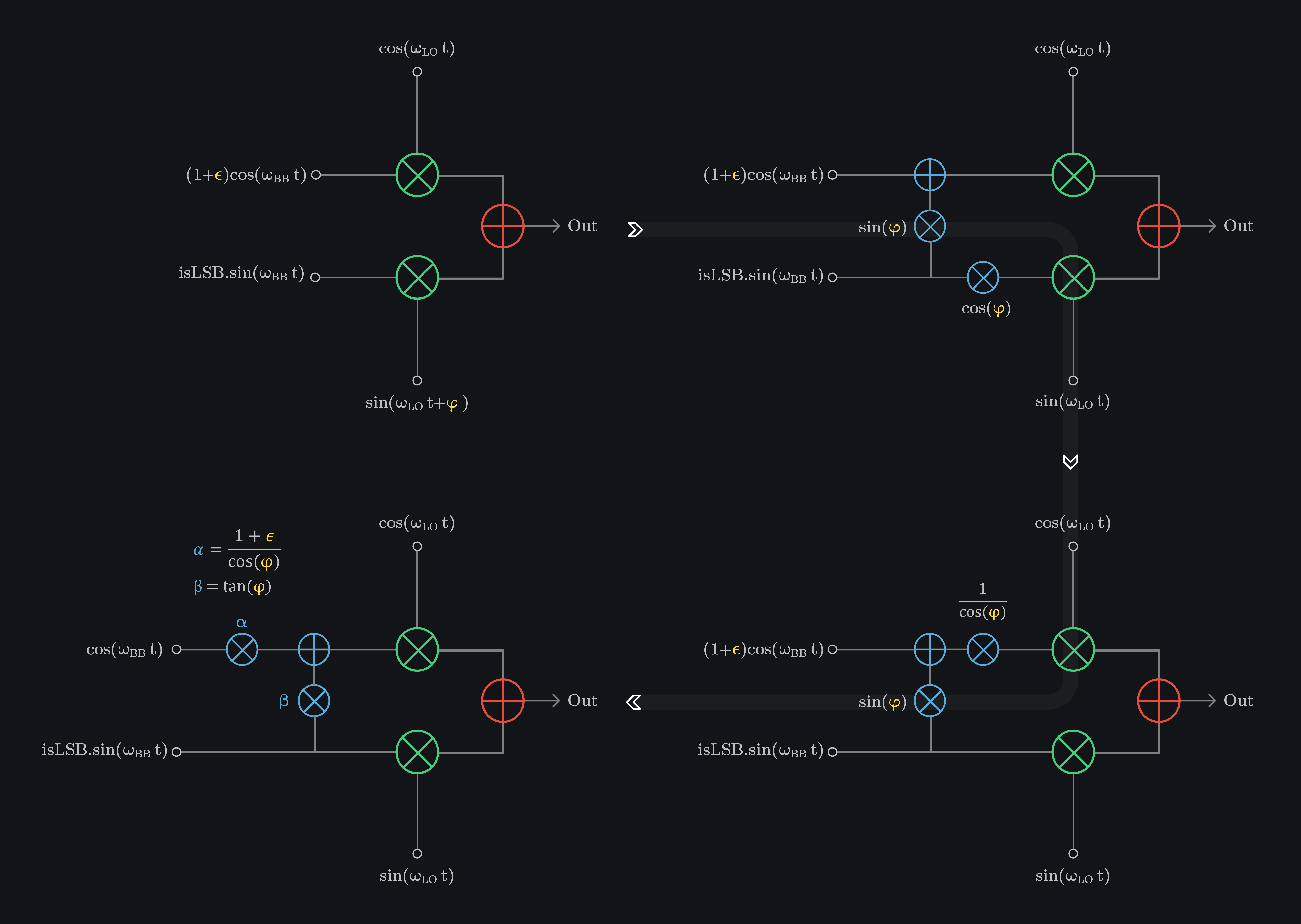
so our IQ TX with gain and phase errors is equivalent to figure in bottom left that is we can model gain and phase errors by gain scaling \(\textcolor{#57ACDC}{\alpha}\) and IQ cross talk \(\textcolor{#57ACDC}{\beta}\).

\textcolor{#57ACDC}{\alpha} = \frac{1+{\large \textcolor{#FEDB39}{\epsilon}}}{cos(\textcolor{#FEDB39}{\varphi})}\;\;\;\text{&}\;\;\; \textcolor{#57ACDC}{\beta} = tan(\textcolor{#FEDB39}{\varphi})

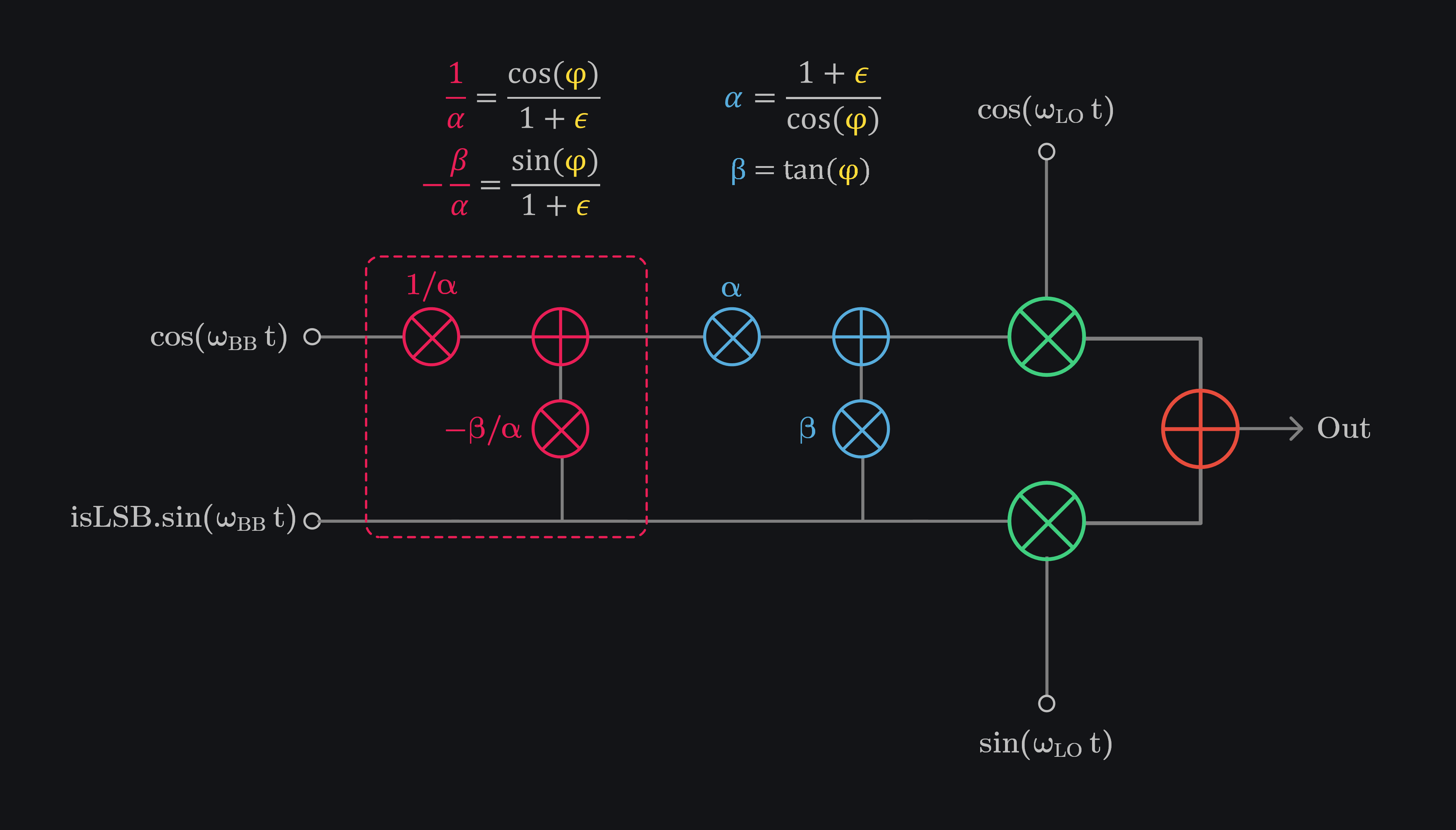
We can calibrate the errors by doing opposite as shown in image below. This circuitry will be added in digital front end where data of I channel will be scaled by \(\frac{1}{\alpha}\) and \(-\frac{\beta}{\alpha}\) of Q data will be added to it. Once this data is send on I channel, it will correct the gain and phase errors of system. We can send the Q data as it is to Q channel, we don’t need to add/multiply anything to it.

Verification of IQ Calibration in Cadence

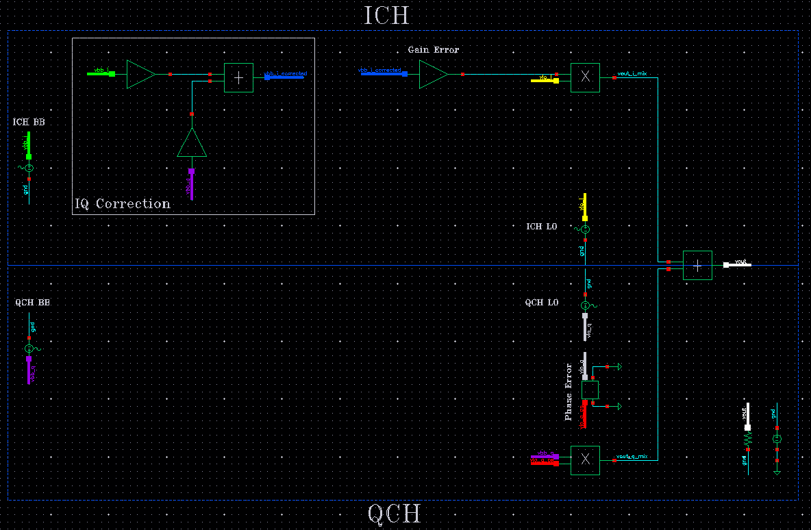
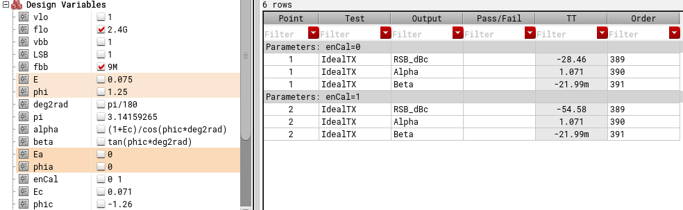
We built an IQ TX in Cadence using ideal blocks like multipliers, summers and delay elements from ahdlLib library as shown in image below.

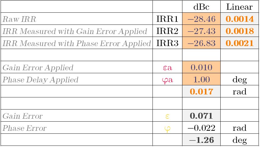
We added gain error of 0.075 to I channel BB and phase delay of 1.25 degree to Q channel LO. Our goal is now get these numbers from calibration algorithm presented above. We measure (or simulate in this case) raw IRR1, IRR2 with gain error of 0.01 applied and IRR3 with gain error of 0.01 and phase delay of 1 degree applied. Three measured numbers are shown in image below.

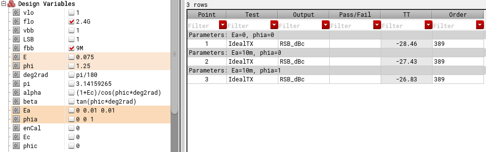
We made an Excel calculator (which is available to download below), plugged these numbers in, and this give us our calculated gain and phase error to be 0.071 and -1.26 degree (means delay). Hmm this is close but does not quite match the actual gain and phase errors in system which were 0.075 and -1.25 degree to be precise.

IRR Calculator

Let’s see what happens when we compute our \(\alpha\) and \(\beta\), and use them for correction of IRR. Image below show IRR before and after calibration.

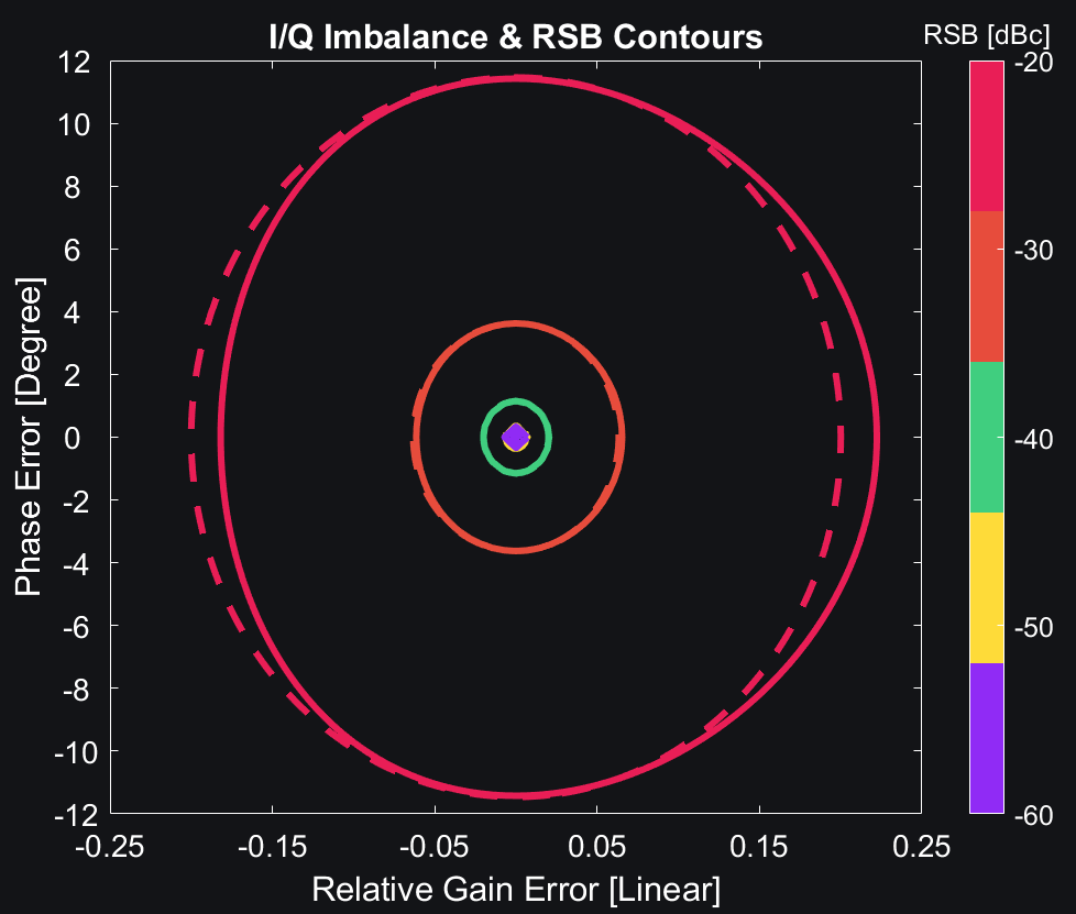
IRR improves from -28dBc to -54dBc after IQ calibration. Good but not perfect. So what is missing? Remember we assumed \({\large \textcolor{#FEDB39}{\epsilon}} <<1\)\( \; \& \; \textcolor{#FEDB39}{\varphi} <<1\), this got us. Our calculator could not calculate exact gain and phase error because of this assumption. If you desire to calibrate IRR much better than -50dBc levels, then you would need to get back to original equation of IRR, and use that to calculate errors (instead of circle equation). This is also the reason we applied very small gain and phase errors (0.01 and 1 degree) so that overall gain and phase error (what we applied + what’s already in system) does not exceed our assumption of \({\large \textcolor{#FEDB39}{\epsilon}} <<1\)\( \; \& \; \textcolor{#FEDB39}{\varphi} <<1\). This is also an issue. Your system might not be able to apply such small gain and phase errors. In that case too, you need use original IRR equation. Calibration algorithm remains same. Excel can solve such equation by numerical techniques (like hit and trial).

Image below plots IRR with circle equation (dotted lines) and actual equation (solid lines). We can already see for gain error of 0.1 or more, the circle equation and actual equation don’t match. However, if gain and phase errors are small (i.e., for intrinsic IRRs better than -30dBc), circle equation is good enough.

References [1] Wideband Digital Correction of I and Q Mismatch in Quadrature Radio Receivers (Hardware Friendly Implementation) https://ieeexplore.ieee.org/document/857556 [2] I/Q Imbalance Calibration in Wideband Direct Conversion Receivers https://ieeexplore.ieee.org/document/7790607 [3] A Low-Complexity I/Q Imbalance Calibration Method for Quadrature Modulator (Calibration Algorithm) https://ieeexplore.ieee.org/document/8576561

Appendix

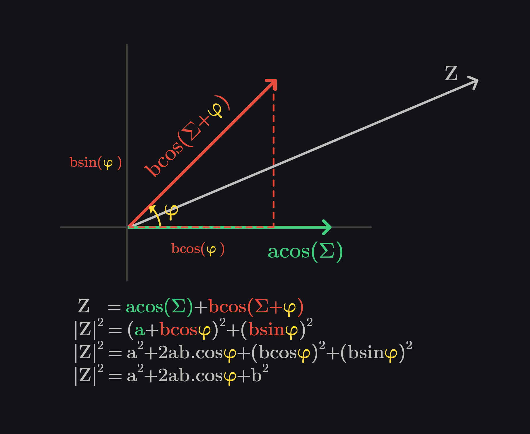
Summation of two vectors with phase \(\textcolor{#FEDB39}{\varphi}\) between them.

Assume a vector \(acos(\Sigma)\) and a scaled phase shifted version of it \(bcos(\Sigma+\textcolor{#FEDB39}{\varphi})\). We show in image below how can we calculate magnitude of their sum (vector Z).

RFInsights

Published: 04 June 2023
Last Edit: 04 June 2023