Transient to Spectrum

In IC design, there comes a time when netlist of a circuit gets too big that harmonic balance (HB) or periodic steady state (PSS) simulations just would not converge or take eternity to finish. It is then we resort to classic time domain transient (tran) simulation where convergence is almost always guaranteed but converting that time domain signal to frequency domain brings a lot of frustration and skepticism as to whether FFT results are correct or not. In this article, we will cover how to take FFT in Cadence and what to watch out for.

Top Three Mistakes in FFT

You did not low pass filter your signal, you suffer from aliasing.
You did not sample integer number of cycles, you suffer from spectral leakage.
You did not add strobe period in tran sim, you suffer from interpolation error.

FFT in Cadence

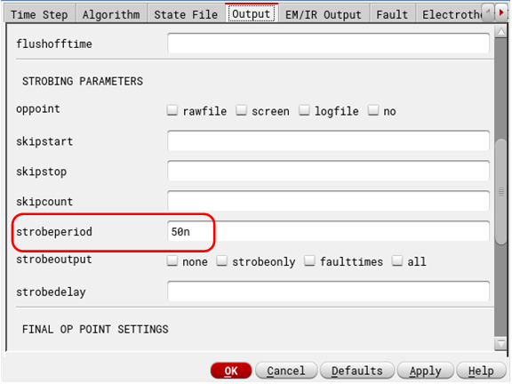
1. Decide Maxium Frequency – Set Strobe Period

Your signal might have infinite frequencies in it but you cannot have infinite sampling rate to capture them. Decide maximum frequency ($f_{max}$) you are interested in, and set sampling rate ($f_{s}$) twice of that. Say, $f_{max} = 10 MHz$
$$ f_{s} = 2\times f_{max} = 2 \times 10 MHz = 20 MHz$$
$$ T_s = \frac{1}{f_s} = \frac{1} {20MHz} = 50 nS$$

Your sampling period ($ T_s $) will be your strobe period ($ T_{strobe} $) in Cadence tran simulations. Strobe period defines step size in tran simulations, and you want to make sure the points you are going to be sampling at (which are $ T_s $ apart) are actually simulated, not interpolated. To err on side of caution, I make sure my $T_{strobe} $ is 10 times lower than $ T_s $ (maybe an overkill if your simulation time explodes).

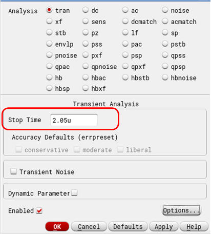
2. Decide Frequency Resolution – Set Simulation Time

The Transient simulation time ($T$) is inversely proportional to the desired frequency resolution ($f_{res}$). Decide what $f_{res}$ you can afford, this will also set the lowest frequency you can analyze. Say, $f_{res} = 1 MHz$ $$ T = \frac{1}{f_{res}} = \frac{1}{1MHz} = 1uS$$ You need to sample your signal once transient has settled and it has reached steady state, lets call that time $t_{settle}$. It is also wise to also add some margin at end of signal just as a precaution, lets call that time margin $t_{margin}$. Say, $t_{settle} = 1uS$ and a $t_{margin}$ of 1 sample i.e., $ t_{margin} = T_{s} = 50nS $. This makes your total simulation time to be: $$T_{sim} = t_{settle}+T+t_{margin} = 1uS + 1uS + 0.05uS = 2.05uS$$

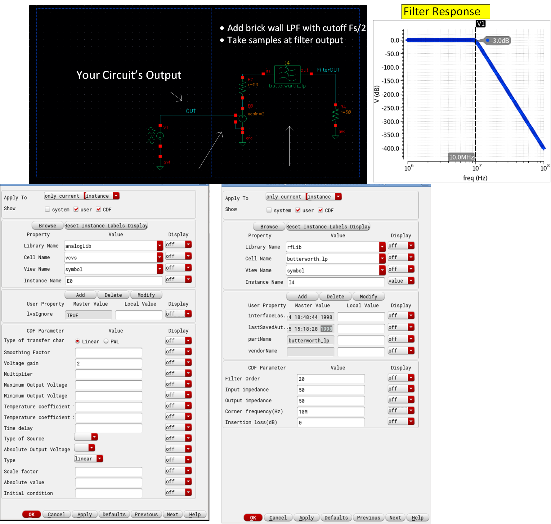
3. Add Low Pass Filter

Your FFT will suffer from aliasing if you do not low pass filter (LPF) your signal before you sample it. Aliasing will fold any frequency beyond $\frac{f_s}{2}$ to your desired band $(0-f_{max})$ which means your FFT will show you frequency components which are not actually there, rather artifacts of FFT. Therefore, you really want to add an ideal brick-wall LPF to make sure there is no aliasing.

Note that I have a vcvs of gain 2 that is because filter needs to be terminated with $50\Omega$ at input and output. At input, it will divide the signal by 2, to recover that I add gain of 2. Also, note that this filter is modelled in s-domain, if input signal is barely just sampled enough for your needs, that might not be enough for this filter (meaning you need to reduce $T_{srobe}$ which was set to $T_{s}$). Try with $T_{strobe}=T_{s}$ and $ T_{strobe} = 0.1 \times T_{s} $ and see the filter output signal in time domain. If there is a difference, go with lower $T_{strobe}$.

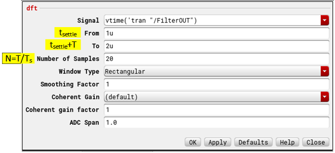
4. Use DFT Function

The number of FFT points equal to number of samples you take which is: $$ N = \frac{T}{T_s} = \frac {1uS}{50nS} = 20 $$

Leave rest of the options default that is no fancy window (just plain Rectangular Window); no Smoothing Factor or Coherent Gain since we use Rectangular Window (other windows changes the signal’s amplitude, you use coherent gain to correct that); no ADC span (specifies the peak saturation level of the FFT waveform. When specified the magnitude of the input waveform is divided by adc span value before computing FFT).

Convert the output to dB using dB20( ) if you would like. Final expression would look like:

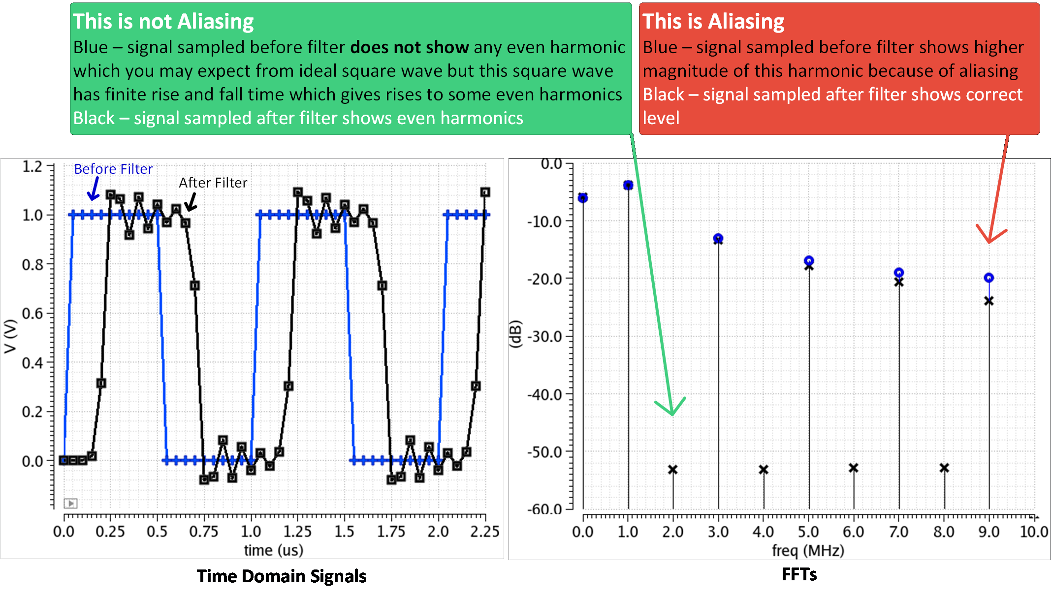
Your FFT is all ready. Compare it before and after the filter just for fun. My input signal is 1MHz square wave with 1nS rise/fall time. Which FFT is correct? (hint: the one after filter).

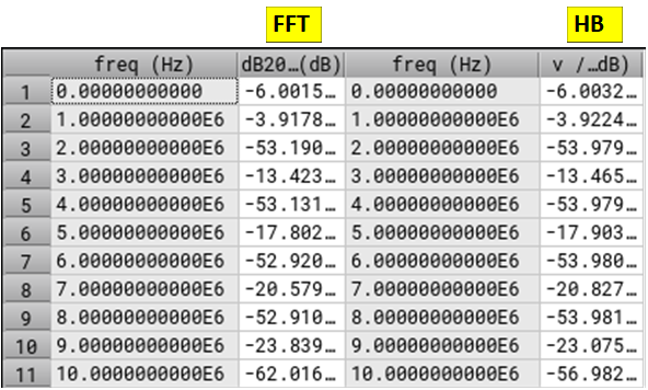
When compared with Harmonic Balance, FFT matches pretty well. However, we do see that as we go to higher harmonic, HB and FFT start to differ a little. Why is that? Two things:

Our filter’s corner frequency is 10MHz, so it is adding 3dB attenuation as you approach 10MHz
Filter is not really brick-wall, 11MHz harmonic is only getting 17dB attenuation, so it will fold and corrupt 9MHz. What do we do now? Increase sampling rate. Say you really want to see precise magnitude of 10MHz, then you can double sampling rate, thereby also doubling filter cutoff. This way 10MHz won’t have aliasing or filter attenuation but 20MHz would (Have you grown sudden care for 20MHz now?)

5. Phew, Ok Great, Was that all?

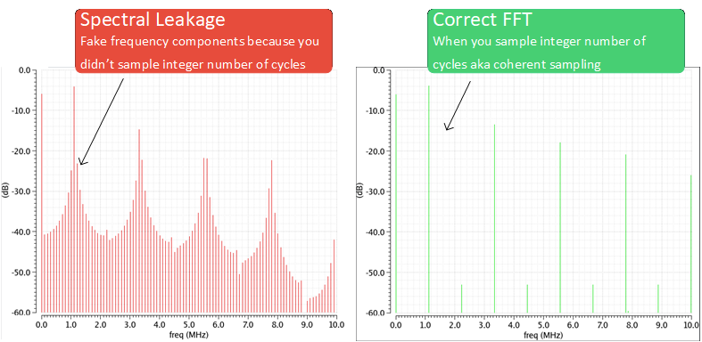
Afraid not. One more thing that you need to watch out for is coherent sampling. When you take DFT, it implicitly assumes that time sample blocks repeat every N samples which means if you did not sample over complete cycle of your signal, you messed up spectral leakage. Imagine you only sampled half sin wave, you give that samples to DFT, it will think “hmm, so signal is half sin wave and repeating, I see its a full rectified sin wave”. Amm, no, its just a sin wave. You better give DFT samples of full sin wave cycle so that when it “cascades” sin wave they still look like sin waves. Don’t believe me? See below. I just changed my signal frequency from 1MHz to 1.11MHz and increased $f_{res}$ to 0.1MHz just to emphasize spillage. You see how 1.11MHz has grown big side-lobes, this is called spectral leakage. These are fake. Imagine if you were trying to debug whether there is a frequency component near 1.11MHz or not, you see this spectrum and you might think you found it but you would be wrong as it was fake. You can either use windows to get rid of them (good luck), or sample integer number of cycles.

Sample at Integer Number of Cycles

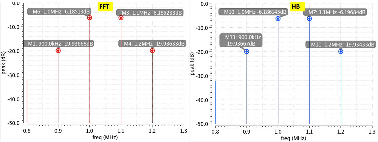
If your signal is just one sin wave, you can sample over integer number of cycles. No problem, done deal. What if your signal is composed of lots of sinusoids, which sinusoid would you sample at integer cycles? The short answer is all. Take greatest common divider (GCD) of all the frequencies you are intersested in correctly decoding and sample integer cycles of GCD frequency. This means, go back to step#2 and choose $f_{res}$ to be $f_{GCD}$.
$$f_{res} = f_{GCD}$$
Say we are doing IM3 test. We excite our circuit with 2 tones (1MHz,1.1MHz), our IM3 tones will fall at (0.9MHz,1.2MHz). The tones we are interested in measuring correctly are (0.9MHz,1MHz,1.1MHz,1.2MHz). GCD of these tones is 0.1MHz. If you sample 0.1MHz coherently (meaning sample integer number of cycles), you will be sampling all these (0.9MHz,1MHz,1.1MHz,1.2MHz) coherently as well. And now to sample 0.1MHz coherently, you need to set $f_{res}$ to 0.1MHz.
We had 1MHz $f_{res}$ before which gave us 1uS sim time, but now with 0.1MHz $f_{res}$, sim time has increased to 10uS, that is the price we paid. To get around this, consider changing your input frequencies to say (1MHz,2MHz). Now GCD is 1MHz, so your $f_{res}$ won’t have to change.

Tips to Debug FFT

Increase sampling rate, if you see differences, there is still some aliasing at play.
Reduce frequency resolution, if you see differences, there is still some spectral leakage at play.
Decrease strobe period beyond sampling period, if you see differences, there is something wrong with simulation accuracy or things in your circuit which are modelled in frequency domain (like s-parameters, low pass filter model described above etc.)
Done everything, still see spectral leakage? Time to start applying windows. Start with Hamming, Hanning and Blackman windows. Observe how windows are changing your FFT. Things that don’t change with windows are very likely real. Things that change were likely FFT artifacts. Small changes in amplitudes, here and there, are expected with windows, we are looking for big changes.