Semiconductor Yield Estimation
“Hey relax this spec please. I tried everything. It is what it is. If you do not relax now, you will see big yield loss (when we eventually go for large data collections, and that stage might come very late in project cycle), so don’t come charging at me then, I warned you my estimated yields are not looking good based on current specs.”
Ok, so how do we make semiconductor yield estimation and what jargons do you speak? Let’s take a dive.
CPK
Process guys usually think of yield in terms of CPK (process capability index). It was designed to show how well the process is doing given its part performance. They designed a process, observed its spread of say gate thickness and came up with standard deviation number. Now, next time when they produce wafers with same process, they were like: “hmm I wonder if this process is still any good, if it is still capable“. Thus, they came up with this CPK index to give them a sense of how process is doing. They could have just checked the standard deviation again, but no they had to define a new index for them, and now we IC designers also are asked to use it, oh well. The CPK, standard deviation or % yield they are just different ways of saying how many parts are failing.
Let’s try to understand this formula a bit. Say you an amplifier and it has spec on the lowest gain it can have (LSL), and on high side it can be as high as it gets (USL can be infinite). So right part of the formula can be ignored. Now the concept here is to see how far your LSL is from mean, and compare it with 3\(\sigma\). Say if your LSL is 3\(\sigma\) away, CPK becomes 1. So then CPK=1 means your parts are within +/- 3\(\sigma\) which is great, CPK=2 means your parts are within +/- 6\(\sigma\) which is out of this world. A faster way to calculate \(\sigma\) from CPK is to just multiply CPK by 3.
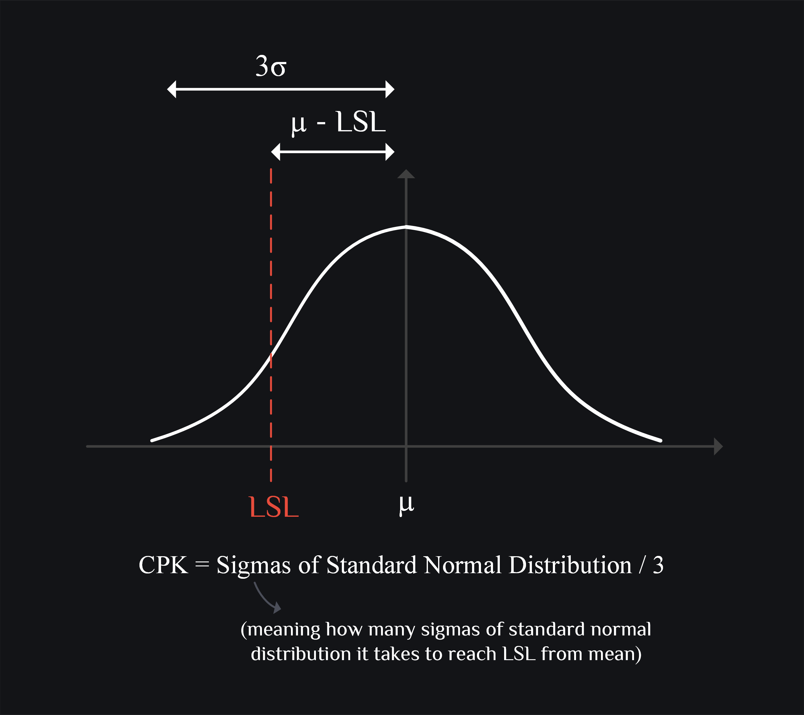
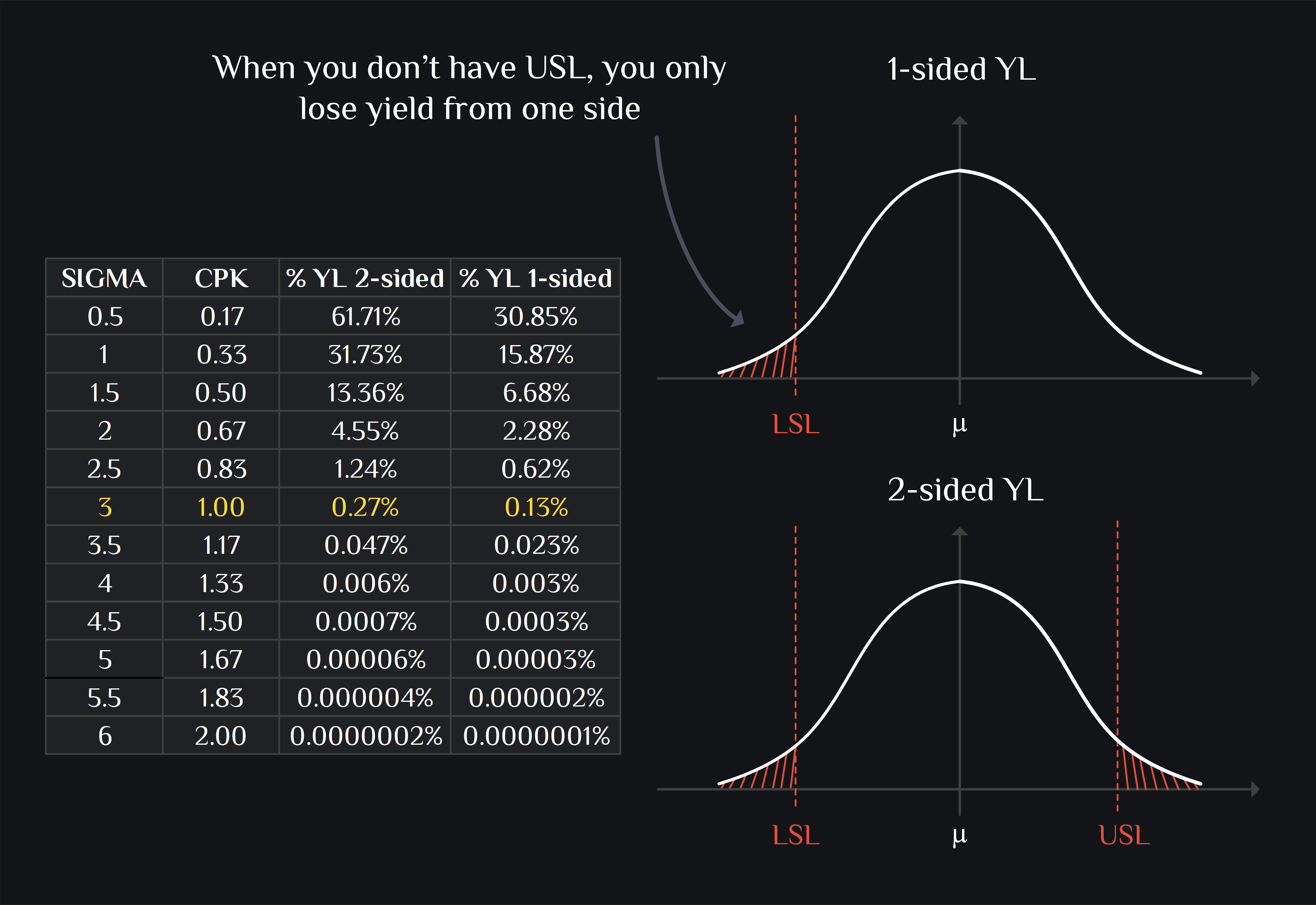
Ok, good to know CPK but still % number is more intuitive. How do I know % yield loss? If you wanna do this in your head, you would multiply CPK with 3 to get \(\sigma\), and you would recall +/- 3\(\sigma\) means 99.7% (i.e., only 0.3% yield loss), +/- 2\(\sigma\) means 95% (i.e., 5% yield loss) and +/- \(\sigma\) would mean 68% (i.e., 32% yield loss). Please see below section for more generalized way.
Yield Estimation
CPK is derived for normal distribution which is symmetric around its mean. Most of the numbers we measure are in dB which have asymmetric distribution (aka skewed). You have two options:
1. Convert dB to Linear and use Normal Distribution Statistics
Your skewed distribution would become normal when you convert it to linear scale. You can either use factor of 10 or 20, does not really matter. I use 20:
Parameters like ACLR, LO leakage and image rejection etc. with skewed distribution in dB scale transform into normal distribution in linear scale. So now you can apply normal distributions statistics to get yield estimate. Before that, you standardize your data (meaning make its mean equal to zero, and standard deviation one), plot it and then start integrating from -inf until you reach your LSL. The area under the curve would be the probability of parts that failed. Microsoft Excel can do these both steps with one command:
If you have LSL: NORM.DIST(LSL , \(\mu\) , \(\sigma\) , TRUE)
If you have USL: 1 – NORM.DIST(USL , \(\mu\) , \(\sigma\) , TRUE)
If you have both LSL & USL: 1 – NORM.DIST(USL , \(\mu\) , \(\sigma\) , TRUE) + NORM.DIST(LSL , \(\mu\) , \(\sigma\) , TRUE)
2. Model Skewed Distribution to Normal Distribution
If you are insistent on using your data in dB, and you see already it is forming a skewed distribution, you still have a hope. You cannot compute \(\sigma\) for skewed distribution like you used to do for normal (take difference from mean and average it in RMS fashion) because if you do, that would not truly represent your data.For example, say you distribution is positively skewed (meaning it has really long right tail), your +/- 3\(\sigma\) would say you have covered 99.7% of parts but you wouldn’t have because God knows how long that tail is going to be. In this case, your best bet is to come up with a pseudo sigma (\(\sigma_s\)) with which you can still apply normal distributions statics and confidently say yes now +/- 3\(\sigma_s\) have covered 99.7% of parts.
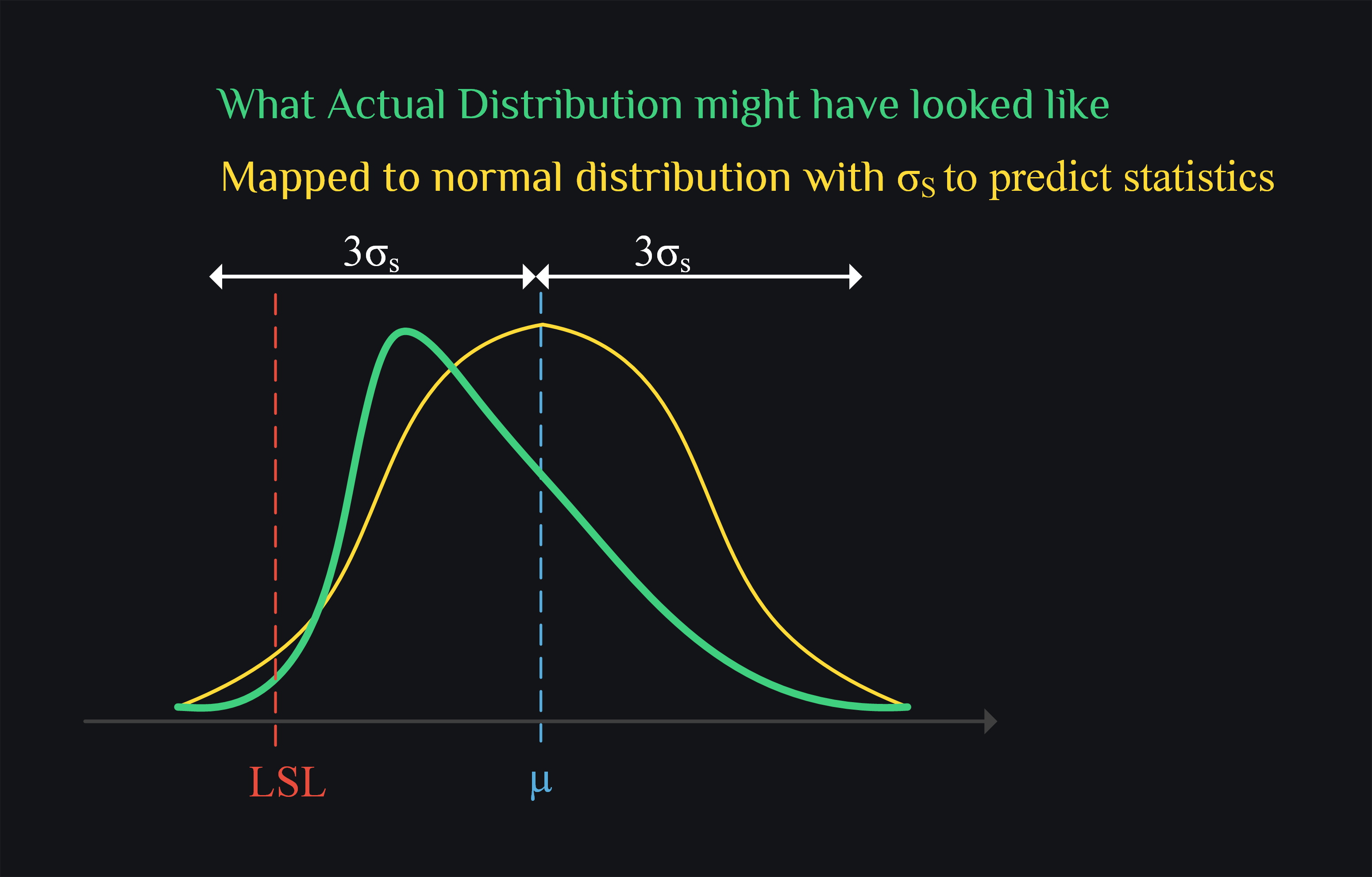
Now how do you come up with \(\sigma_s\). You can take help from percentiles. For example, in standard normal distribution, 5th percentile lies at -1.6\(\sigma\) away from mean. How did I know this? you can integrate your standard normal distribution from -inf uptil you have accumulated 0.05 probability which means 5% of parts or in other words 5th percentile. You don’t want to integrate? No problem, there are tables available already online called z-tables, you can figure out for 0.05 probability what is z-score, and that z-score will mean you are this much \(\sigma\) away from mean. Now all you need to do is to compare mean – 5th percentile of your data to z-score (which is 1.6 for 5th percentile). If mean- 5th percentile is also 1.6, then it means your distribution is already standard normal with \(\sigma_s=\sigma=1\). Here is the general formula for pseudo sigma:
How do you go from here? Use linear yield estimate. If your distribution is still skewed, model it to normal distribution by \(\sigma_s\).
Example and Excel Calculator
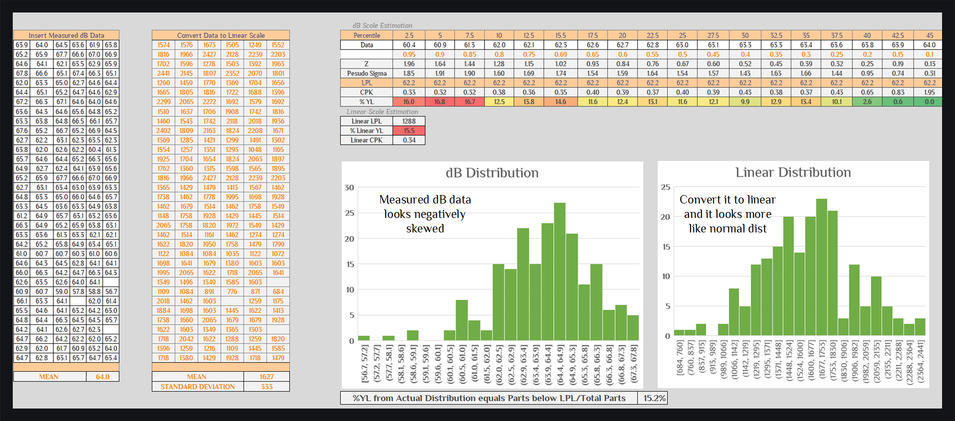
We show below some dB data with negatively distribution skewed. We have LPL spec of 62dB. About 200 parts were measured. Yield was calculate in three ways: by actually counting the parts which were failing (15.2%), by converting dB to linear and using normal statistics (15.6%), by estimating pseudo sigma using 5th percentile (16.8%). We see linear estimation is spot on and dB estimation is little off. We would trust 15.6% over 15.2%, why? because parts measured are still on low side (200, not millions). We also show how would dB estimation look like if you had chosen different percentiles.
Author: RFInsights
Date Published: 18 Dec 2022
Last Edit: 02 Feb 2023