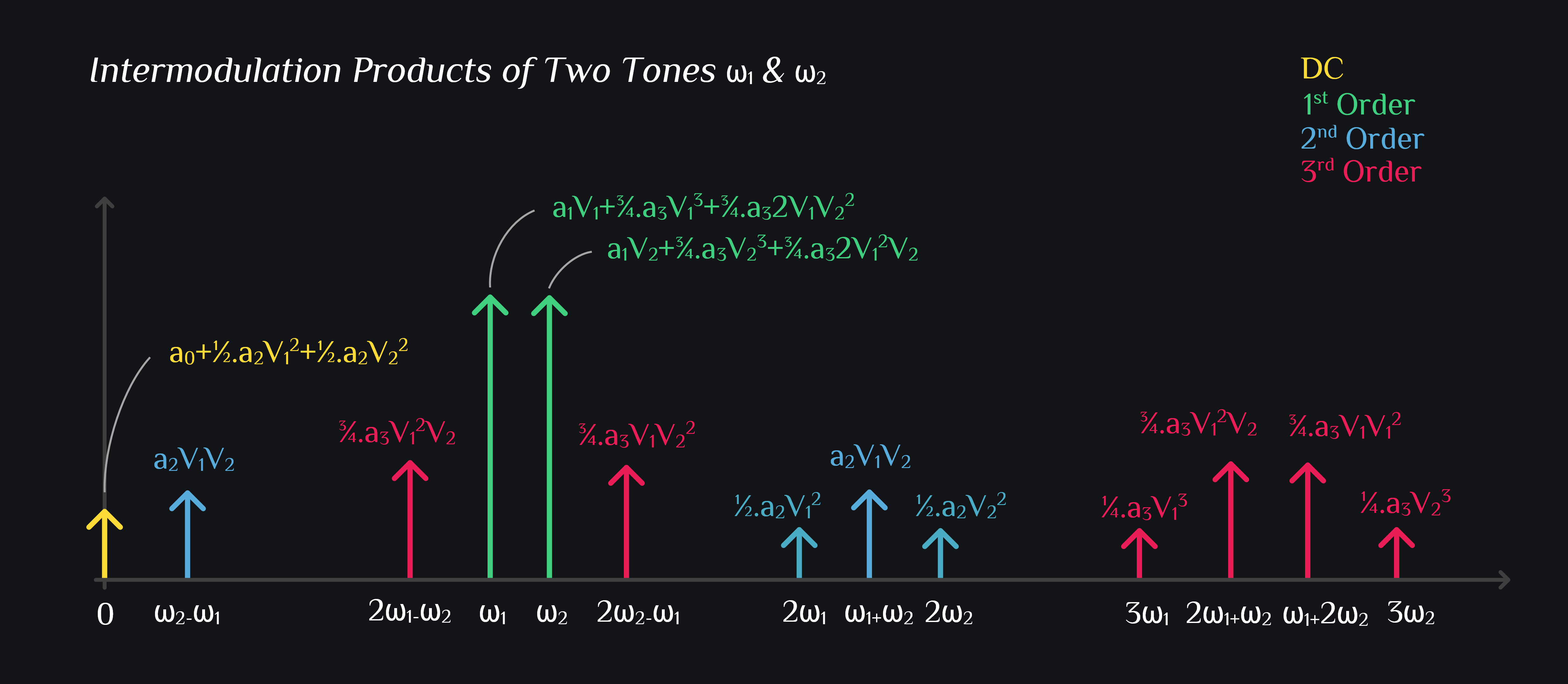
Intermodulation of Two Tones
Admit it. You are lazy and don’t make notes. You do this math every time you need to remember what distortion products are generated by intermodulation of two tones and what is their relative level. No more. We are doing the math now, so you don’t have to.
Intermodulation Math
Assume a non-linear system whose output has up to third order of non-linearity. We can relate output and input as:
Lets excite this system with two tones:
Output can be written as:
Expanding Terms
Square terms:
Cubic terms:
Collecting Terms
DC
How interesting. 2nd order non-linearity can generate a DC term proportional to signal. Fortunately, our systems are differential implying \(a_2=0\) for all practical purposes.
Signal
Lets breakdown this sum.
- You have \(a_1V_1\) which says your \(V_1\) signal goes into the system, gets scaled by \(a_1\) and comes out.
- You have \(\frac{3}{4}a_3V_1^3\) which says cubic distortion of your system also generates fundamental component (yes, cubic distortion did not just generate an intermodulation product, but your signal as well, hmm). Sign of \(a_3\) determines whether it is a compressive non-linearity or expansive. Typically our systems are compressive because voltage or current clips at some point, so \(a_3\) is negative. That means as \(a_3V_1^3\) becomes bigger and bigger, your output signal goes smaller and smaller. That is right. At one point, you will see your signal has reduced by 1dB compared to what it was before when \(a_3V_1^3\) was small (rings the bell? the famous P1 dB point)
- You have \(\frac{3}{2}a_3V_1V_2^2\) which says \(V_2\) also generates some signal at \(\omega_1\) frequency. If \(V_2\) were zero, we wouldn’t have this term and if \(V_2\) were very big, it will dominate the total sum and you wouldn’t see your nice \(a_1V_1\) signal anywhere. This is called desensitization. This happens in receivers where a jammer (just like \(V_2\) here) desensitizes your receiver. By same token, if \(V_2\) is amplitude modulated, it will transfer its modulation at \(\omega_1\) frequency too, called cross-modulation. Being nit picky here: phase modulations are not transfered.
2nd order Intermodulation Products
Now this is a rather nasty yet easily ignored product, with designers thinking that it lies far away from our signal. We also call it beat or envelope frequency because if you look at envelope of your signal \((\omega_1+\omega_2)\), it will be moving slow at beat frequency. It is important because it also generates IM3 from “2nd Order Interaction” which basically means 2nd order IMD products from 1st stage when subject to non-linearity of subsequent stages end up producing IM3. Lets make it simple. Say you have a driver amplifier followed by power amplifier. Driver amplifier receives two tones at input, and generates all the intermodulation products. Now all of these are input to power amplifier. Consider intermodulation of \(\omega_2-\omega_1\) with \(\omega_1\) & \(\omega_2\). This will generate \(2\omega_1-\omega_2\) & \(2\omega_2-\omega_1\) terms, which are IM3 frequencies. See how 2nd order non-linearity of 1st stage caused IM3s. Ok, big deal. Another source of IM3, so what? Yes, big deal. This source of IM3s is poorly controlled by designers. It creates asymmetrical and tone spacing dependent IM3 (heard of memory effects?). Also note that its not just beat frequency, \(2\omega_1\) & \(2\omega_2\) also manifest similar phenomena, however they are not given much importance because they already lie at high frequencies and get somewhat low pass filtered before making it to subsequent blocks.
3rd order Intermodulation Products
These are the IM3 terms. Consider the first term (left IM3). Factor \(V_1^2V_2\) tells you that IM3 rise 3dB for every dB increase in \(V_1\) and \(V_2\). What about if you only increase one of the signal, say \(V_1\). That is a famous interview question. We can see if \(V_1\) increases by 1 dB and \(V_2\) remains constant, left IM3 would increase by 2dB where as right IM3 would increase by 1dB.
Author: RFInsights
Date Published: 11 Oct 2022
Last Edit: 02 Feb 2023